Project goal

Build a GenAI-driven classification system to audit and improve how a public, internationally adopted taxonomy is applied at scale, across millions of real-world records, where labels are expert-defined, ground truth is imbalanced, and small error rates can translate into large downstream impact.

MLOps goal (the way we work)

Treat experimentation discipline as part of how the team operates, not as a tooling layer. From the start, this meant being explicit about success criteria, tracking conflicting objectives (quality, cost, and performance) side by side, versioning parameters and prompts, and closing fast feedback loops. Decisions were communicated using data and reproducible runs, not opinions or sales narratives. Tools like spreadsheets or MLflow were implementation details; the real value came from consistency, traceability, and making change observable over time.

Where we started

We started with a naive POC and then evolved it into an MVP with a multi-stage GenAI classification pipeline. Functionally, it worked. Measured against real constraints, it was expensive, slow, and difficult to reason about:

• Quality: precision and recall were uneven, with acceptable recall but low precision, making it hard to trust outputs at scale
• Cost: early approaches cost on the order of ~$0.15–$0.25 per record
• Performance: end-to-end processing time was measured in minutes per record

At that stage, these numbers were not surprising—they were typical for a first GenAI POC. What mattered was that they were measured, written down, and treated as a baseline rather than hand-waved away.

Operationally, several critical questions remained unanswered. The changes that followed made a systematic, disciplined method unavoidable.

The two real challenges

1. The GenAI system was complex by design

This wasn’t an AI wrapper or a single prompt. It was an advanced, agentic pipeline where each stage shaped the next:

1. GenAI filtering: remove weak/ambiguous inputs and narrow the search space.
2. Feature amplification: use language models to enrich sparse descriptions into higher-signal text/features.
3. Vector retrieval: generate candidate labels/codes from a large taxonomy.
4. LLM reranker: decide among top-K candidates and output the final prediction.

That architecture improved performance, but it also made cause-and-effect harder. A tiny change upstream could create a surprising downstream “ripple”.

2. Imbalanced data (a known problem with sharper edges at scale)

Data imbalance itself wasn’t novel. What mattered was its interaction with scale and multi-stage GenAI decisions. With most records already correct, small shifts in precision vs. recall could look harmless in percentages while translating into large absolute counts downstream. Rather than collapsing system behavior into a single headline metric, we examined precision, recall, and F1 together with running cost and processing latency, and looked at how all of them moved as the system changed. The goal was not to optimize any metric in isolation, but to understand why a change improved one signal, degraded another, and how those shifts translated into real cost and performance impact at scale.

Why experiment tracking became non-optional

Once we had multiple interacting components, ad-hoc iteration broke down.

When quality changed, we needed to know whether it was caused by:

• embeddings / dimensionality
• vector store choice (and its similarity implementation)
• distance function (cosine vs dot product / normalization behavior)
• hybrid search weighting
• top_k candidate count
• filter thresholds
• prompt versions (filter and reranker)
• reranker decision rules

Without systematic tracking, we risked:

• attributing improvements to the wrong change
• shipping regressions masked by imbalance
• “optimizing” cost in a way that silently reduced quality

So we made every run auditable and replayable.

How we bootstrapped MLOps before tools

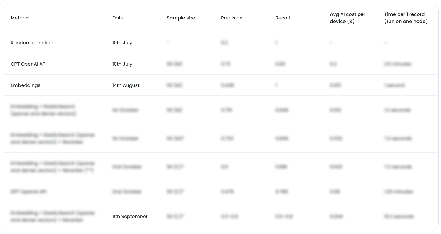
Before introducing MLflow, we used a shared Google Doc/Sheet as a lightweight experiment ledger. Over the course of several development iterations, this allowed us to run dozens of experiments in a controlled way—enough to explore the design space, but with meaningful manual overhead. It was intentionally simple, but highly structured:

• One row per experiment (date-stamped)
• Method / pipeline variant (e.g. baseline, embeddings, hybrid retrieval, reranker, filtering strategy)
• Sample size (small expert-curated sets vs. larger confidence samples)
• Quality metrics: precision and recall (and later F1), always measured end-to-end
• Cost metrics: average AI cost per record (USD), derived from token usage
• Performance metrics: processing time per record, measured on a single node for consistency

Notes: hypothesis, what changed vs. previous run, and known caveats

Crucially, we tracked these dimensions together, not in isolation:

• improving precision while recall dropped was recorded explicitly
• cost reductions were only accepted if quality stayed within bounds
• faster runs were flagged if they coincided with quality regressions

This made trade-offs visible early. Instead of debating opinions, we compared rows. Instead of asking “is this better?”, we asked “better in which dimension, and at what cost?”. Just as importantly, this structure dramatically improved innovation and collaboration: stakeholders could see unbiased results evolve over time, understand the consequences of changes without our interpretation layered on top, and engage in clear, data-oriented discussions. That transparency became a turning point in how we worked together.

Snapshot: how the system evolved over time

The table below illustrates the shape of progress rather than exact values. It highlights the entry point, an intermediate milestone, and the stabilized state—along with where the shift from document-based tracking to MLflow unlocked a higher experimentation cadence.

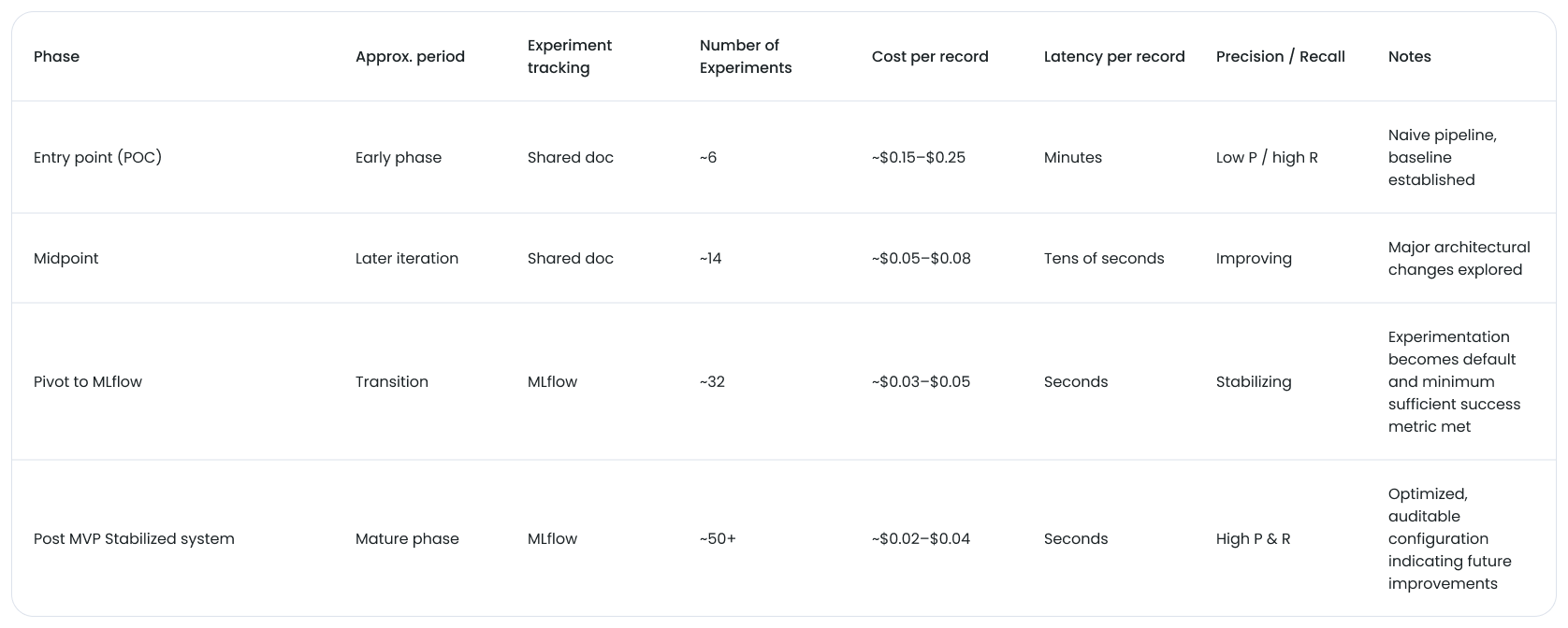
The key inflection wasn’t a single winning experiment. It was the point where experimenting accelerated. Once experiment tracking friction dropped, we could run more experiments with less effort, making learning faster and decisions safer.

From Google Docs to MLflow: Making ripple effects visible

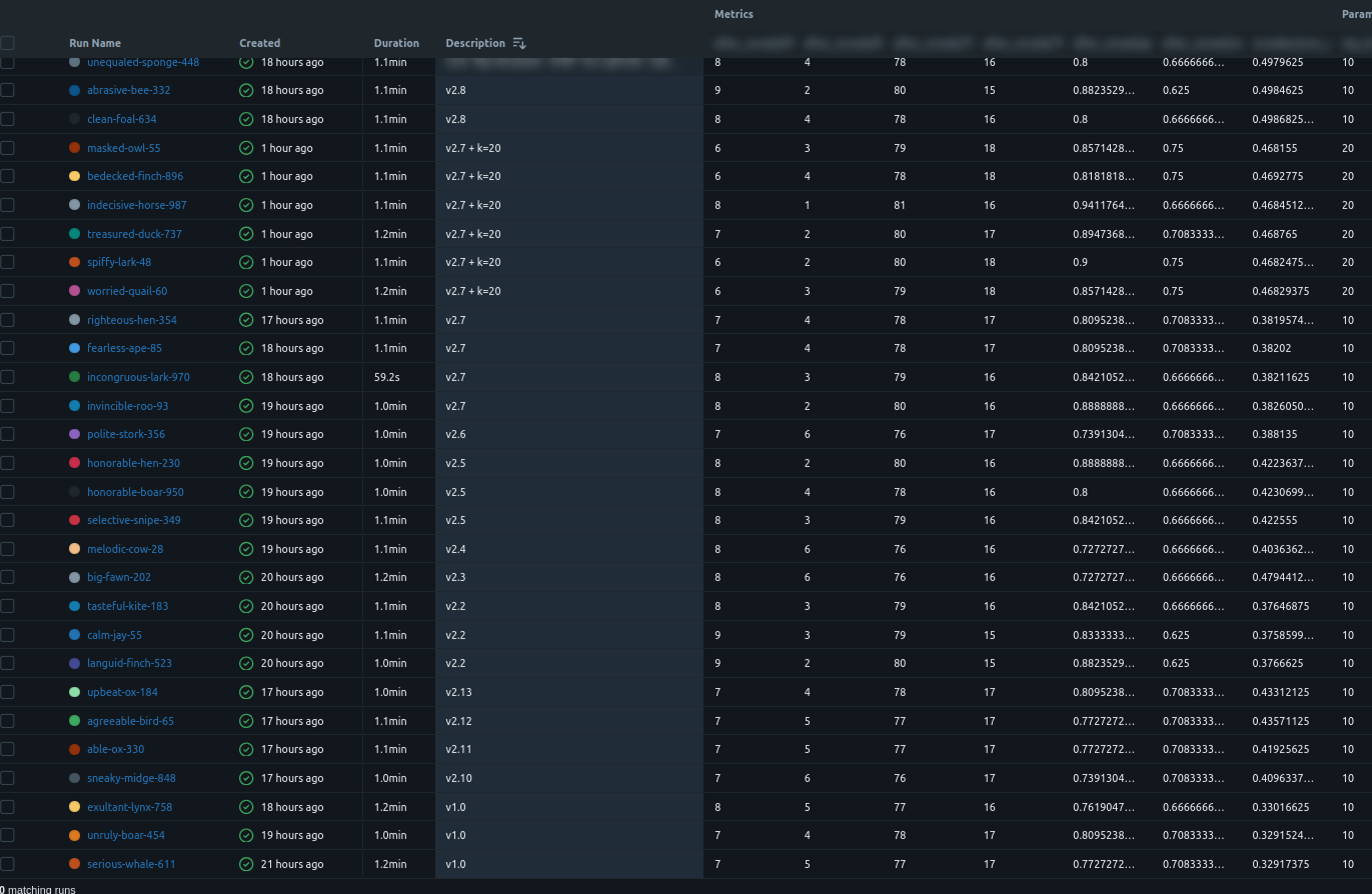
MLflow experiment comparison view showing parameters, metrics, and cost side by side.

As the experiment volume grew, we moved from manual tracking to MLflow. With the discipline already in place, this shift made experimentation the default: instead of running tens of experiments over multiple iterations, we could now run and compare experiments continuously, with far lower friction. MLflow allowed us to:

• log parameters for every stage (retrieval + prompts + thresholds)
• log metrics consistently (before/after rerank, cost, tokens)
• compare runs side-by-side
• reproduce results and explain decisions

Key idea: MLflow didn’t just store numbers. It made the system debuggable, auditable and versioned. No experiment was ever lost, overwritten, or backfilled later. Each run existed as a concrete artifact with explicit parameters and measured outcomes, eliminating human error and hindsight bias. Because experiments were versioned and comparable, we could deliberately choose configurations optimized for different business priorities (e.g. higher precision vs. higher recall) without re-running history or reinterpreting results.

A staged optimization strategy to avoid combinatorial explosion

Tiny code sketch (illustrative):

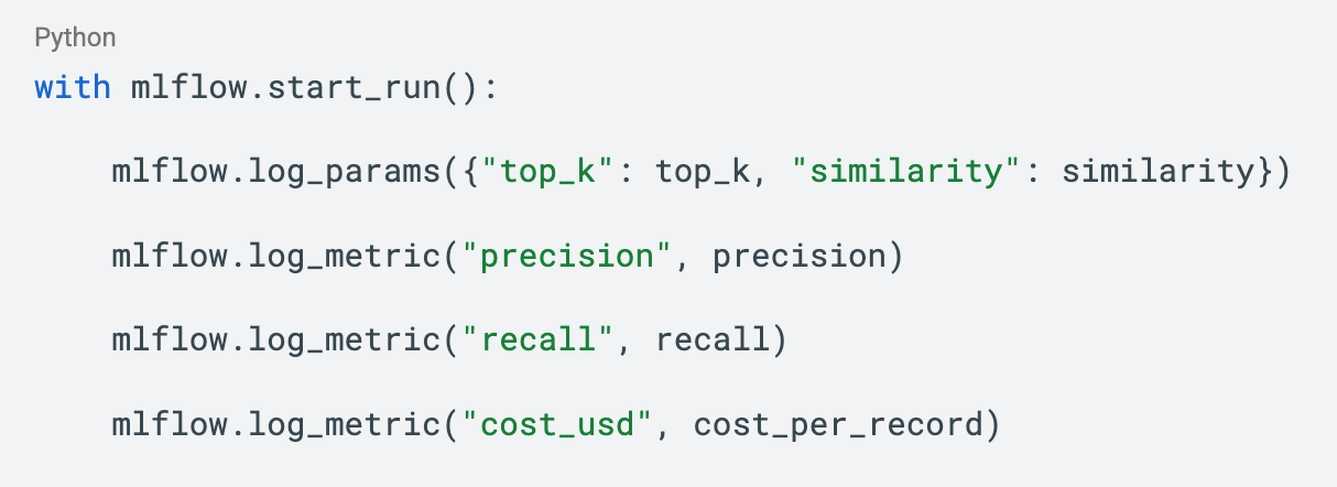
The code itself is trivial. The discipline around when and why it is called is what mattered.

Testing “everything” is unrealistic when you have many knobs. We used a staged approach:

Phase 1: Retrieval optimization (cheap)

• vary retrieval knobs (e.g., hybrid weighting, top_k, similarity)
• keep LLM steps mocked/cached where possible
• measure retrieval and downstream proxy metrics

Phase 2: Prompt and reranker optimization (targeted)

• lock the winning retrieval configuration
• iterate prompt versions and decision rules
• track variance (repeat runs) and measure end-to-end metrics

This gave us speed and clarity: change fewer things at once, learn more per dollar.

Vector stores, similarity functions, and platform trade-offs

We evaluated different vector store options and observed that retrieval behavior is not interchangeable:

• similarity implementations differ (normalization, scoring ranges, ordering)
• hybrid search behavior varies
• metadata filtering and indexing strategies affect recall and latency

We also considered deployment models:

• Managed cloud: faster setup and ops simplicity
• Self-hosted: more control, potential long-run cost advantages

Because these choices can shift candidate sets (and therefore reranker outcomes), we treated infra choices as experiment variables, not assumptions.

Cost was a first-class metric (GenAI makes it unavoidable)

GenAI introduced a cost curve that grows with usage, so cost had to be measured—not inferred.

By the time the pipeline stabilized, the contrast to the starting point was clear:

• Cost: reduced from roughly $0.20 per record to ~$0.02–$0.04 per record (≈ 10× reduction)
• Latency: reduced from minutes per record to a few seconds per record (≈ 50–100× faster)
• Quality: precision and recall both increased and stabilized, rather than trading one for the other

This outcome matters because these three objectives normally pull in opposite directions. In our case, we were able to improve cost, performance, and quality simultaneously—not by luck, but by measuring each dimension explicitly and understanding how changes propagated through the pipeline.

Early experiments made the cost–quality trade-offs visible:

• a naive, API-only approach delivered acceptable recall but cost ~$0.20 per record and took minutes per record
• moving to embedding-based retrieval reduced cost to ~$0.01–$0.03 per record and brought latency down to seconds
• introducing a reranker increased per-record cost again, but in a controlled and explainable way, trading cents for measurable gains in precision and recall

As the pipeline matured, we tracked cost alongside quality and performance:

• Average AI cost per record: reduced by roughly an order of magnitude from early baselines
• Processing time: reduced from minutes to seconds per record on a single node
• Quality: precision and recall improvements were evaluated explicitly against these gains

This allowed us to optimize LLM usage deliberately:

• reduce unnecessary LLM calls (filter early)
• use caching and mocking during search-stage tuning
• reserve expensive calls for stages where they demonstrably improved precision/recall

Some of the most valuable improvements weren’t incremental. They demonstrated that even strongly competing success metrics can be optimized together—if you measure them rigorously and understand the system well enough to act on the details.

This outcome was not accidental. It required experienced AI engineers who were willing to look past aggregate scores and pay attention to small, often noisy signals—edge cases, metric inflections, and subtle distribution shifts that are easy to dismiss but have outsized impact at scale. That attention to detail, combined with disciplined experimentation, is what ultimately unlocked the gains across cost, performance, and quality.

Why MLflow fit our way of working

By the time we introduced MLflow, the discipline already existed. What we needed was a system that could encode that discipline without changing how we worked.

MLflow fit because it aligned with a factory-style design pattern:

• Easy integration: logging experiments required minimal, non-invasive code changes
• Key–value schema: new metrics (quality, cost, performance, domain-specific signals) could be added incrementally without schema migrations
• Open source by design: no lock-in, transparent behavior, and the ability to run a dedicated deployment per project
• One platform to rule them all: a single place to track experiments, models, metrics, and artifacts across the lifecycle

This made MLflow a natural extension of our existing process rather than a new process to learn.

A deliberate design choice was to keep MLflow optional and loosely coupled. Experiment logging could be enabled or disabled without affecting runtime behavior, keeping production deployments lightweight and stable, with minimal additional dependencies.

It also mattered that MLflow is battle-tested at scale. It is used as the experimentation backbone of large production platforms (including managed offerings such as Databricks), which gave us confidence that the same workflows we used in early experimentation would hold up as usage and stakes increased.

Most importantly, MLflow preserved optionality. Because every experiment was a first-class artifact, we could rapidly respond to changing business priorities by selecting models optimized for different objectives (for example, higher precision vs. higher recall) without re-running experiments or reinterpreting past results.

What we learned

1. In complex GenAI pipelines, intuition is not a test.
2. With imbalanced data, you can “improve” metrics while harming the thing you actually care about.
3. Experiment tracking is the difference between tuning and guessing.
4. Treat cost and latency as a metric from day one.

Closing

GenAI systems evolve fast. Assumptions expire faster.

Our takeaway: measure first, change one thing at a time, and keep every run explainable.